Use Cases for Elasticsearch: Document Store

I'll be giving an introductory talk about Elasticsearch twice in July, first at Developer Week Nürnberg, then at Java Forum Stuttgart. I am showing some of the features of Elasticsearch by looking at certain use cases. To prepare for the talks I will try to describe each of the use cases in a blog post as well.

When it comes to Elasticsearch the first thing to look at often is the search part. But in this post I would like to start with its capabilities as a distributed document store.

Getting Started

Before we start we need to install Elasticsearch which fortunately is very easy. You can just download the archive, unpack it and use a script to start it. As it is a Java based application you of course need to have a Java runtime installed.

# download archive
wget https://download.elasticsearch.org/elasticsearch/elasticsearch/elasticsearch-1.2.1.zip
 
# zip is for windows and linux
unzip elasticsearch-1.2.1.zip
 
# on windows: elasticsearch.bat
elasticsearch-1.2.1/bin/elasticsearch

Elasticsearch can be talked to using HTTP and JSON.When looking around at examples you will often see curl being used because it is widely available. (See this post on querying Elasticsearch using plugins for alternatives). To see if it is up and running you can issue a GET request on port 9200: curl -XGET http://localhost:9200. If everything is set up correctly Elasticsearch will respond with something like this:

{
 "status" : 200,"name" : "Hawkeye", 
 "version" : {
  "number" : "1.2.1",
  "build_hash" : "6c95b759f9e7ef0f8e17f77d850da43ce8a4b364",
  "build_timestamp" : "2014-06-03T15:02:52Z",
     "build_snapshot" : false,
     "lucene_version" : "4.8"
  },
  "tagline" : "You Know, for Search"
}

Storing Documents

When I say document this means two things. First, Elasticsearch stores JSON documents and even uses JSON internally a lot. This is an example of a simple document that describes talks for conferences.

{
    "title" : "Anwendungsfälle für Elasticsearch",
    "speaker" : "Florian Hopf",
    "date" : "2014-07-17T15:35:00.000Z",
    "tags" : ["Java", "Lucene"],
    "conference" : {
        "name" : "Java Forum Stuttgart",
        "city" : "Stuttgart"
    } 
}

There are fields and values, arrays and nested documents. Each of those features is supported by Elasticsearch.

Besides the JSON documents that are used for storing data in Elasticsearch, document refers to the underlying library Lucene, that is used to persist the data and handles data as documents consisting of fields. So this is a perfect match: Elasticsearch uses JSON, which is very popular and supported from lots of technologies. But the underlying data structures also use documents.

When indexing a document we can issue a post request to a certain URL. The body of the request contains the document to be stored, the file we are passing contains the content we have seen above.

curl -XPOST http://localhost:9200/conferences/talk/ --data-binary @talk-example-jfs.json

When started Elasticsearch listens on port 9200 by default. For storing information we need to provide some additional information in the URL. The first segment after the port is the index name. An index name is a logical grouping of documents. If you want to compare it to the relational world this can be thought of as the database.

The next segment that needs to be provided is the type. A type can describe the structure of the doucments that are stored in it. You can again compare this to the relational world, this could be a table, but that is only slightly correct. Documents of any kind can be stored in Elasticsearch, that is why it is often called schema free. We will look at this behaviour in the next post where you will see that schema free isn't the most appropriate term for it. For now it is enough to know that you can store documents with completely different structure in Elasticsearch. This also means you can evolve your documents and add new fields as appropriate.

Note that neither index nor type need to exist when starting indexing documents. They will be created automatically, one of the many features that makes it so easy to start with Elasticsearch.

When you are storing a document in Elasticsearch it will automatically generate an id for you that is also returned in the result.

{
 "_index":"conferences",
 "_type":"talk",
 "_id":"GqjY7l8sTxa3jLaFx67_aw",
 "_version":1,
 "created":true
}

In case you want to determine the id yourself you can also use a PUT on the same URL we have seen above plus the id. I don't want to get into trouble by calling this RESTful but did you notice that Elasticsearch makes good use of the HTTP verbs?

Either way how you stored the document you can always retrieve it by specifying the index, type and id.

curl -XGET http://localhost:9200/conferences/talk/GqjY7l8sTxa3jLaFx67_aw?pretty=true

which will respond with something like this:

{
  "_index" : "conferences",
 [...]
  "_source":{
    "title" : "Anwendungsfälle für Elasticsearch",
    "speaker" : "Florian Hopf",
    "date" : "2014-07-17T15:35:00.000Z",
    "tags" : ["Java", "Lucene"],
    "conference" : {
        "name" : "Java Forum Stuttgart",
        "city" : "Stuttgart"
    } 
}
}

You can see that the source in the response contains exactly the document we have indexed before.

Distributed Storage

So far we have seen how Elasticsearch stores and retrieves documents and we have learned that you can evolve the schema of your documents. The huge benefit we haven't touched so far is that it is distributed. Each index can be split into several shards that can then be distributed across several machines.

To see the distributed nature in action fortunately we don't need several machines. First, let's see the state of our currently running instance in the plugin elasticsearch-kopf (See this post on details how to install and use it):

On the left you can see that there is one machine running. The row on top shows that it contains our index conferences. Even though we didn't explicitly tell Elasticsearch it created 5 shards for our index that are currently all on the instance we started. As each of the shards is a Lucene index in itself even if you are running your index on one instance the documents you are storing are already distributed across several Lucene indexes.

We can now use the same installation to start another node. After a short time we should see the instance in the dashboard as well.

As the new node joins the cluster (which by default happens automatically) Elasticsearch will automatically copy the shards to the new node. This is because by default it not only uses 5 shards but also 1 replica, which is a copy of a shard. Replicas are always placed on different nodes than their shards and are used for distributing the load and for fault tolerance. If one of the nodes crashes the data is still available on the other node.

Now, if we start another node something else will happen. Elasticsearch will rebalance the shards. It will copy and move shards to the new node so that the shards are distributed evenly across the machines.

Once defined when creating an index the number of shards can't be changed. That's why you normally overallocate (create more shards than you need right now) or if your data allows it you can create time based indices. Just be aware that sharding comes with some cost and think carefully about what you need. Designing your distribution setup can still be difficult even with Elasticsearch does a lot for you out of the box.

Conclusion

In this post we have seen how easy it is to store and retrieve documents using Elasticsearch. JSON and HTTP are technologies that are available in lots of programming environments. The schema of your documents can be evolved as your requirements change. Elasticsearch distributes the data by default and lets you scale across several machines so it is suited well even for very large data sets.

Though using Elasticsearch as a document store is a real use case it is hard to find users that are only using it that way. Nobody retrieves the documents only by id as we have seen in this post but uses the rich query facilities we will look at next week. Nevertheless you can read about how Hipchat uses Elasticsearch to store billions of messages and how Engagor uses Elasticsearch here and here. Both of them are using Elasticsearch as their primary storage.

Though it sounds more drastic than it probably is: If you are considering using Elasticsearch as your primary storage you should also read this analysis of Elasticsearchs behaviour in case of network partitions. Next week we will be looking at using Elasticsearch for something obvious: Search.

Goodbye Sense - Welcome Alternatives?

I only recently noticed that Sense, the Chrome Plugin for Elasticsearch has been pulled from the app store by its creator. There are quite strong opinions in this thread and I would like to have Sense as a Chrome plugin as well. But I am also totally fine with Elasticsearch as a company trying to monetize some of its products so that is maybe something we just have to accept. What is interesting is that it isn't even possible to fork the project and keep developing it as there is no explicit license in the repo. I guess there is a lesson buried somewhere in here.

In this post I would like to look at some of the alternatives for interacting with Elasticsearch. Though the good thing about Sense is that it is independent from the Elasticsearch installation we are looking at plugins here. It might be possible to use some of them without installing them in Elasticsearch but I didn't really try. The plugins are generally doing more things but I am looking at the REST capabilities only.

Marvel

Marvel is the commercial plugin by Elasticsearch (free for development purposes). Though it does lots of additional things, it contains the new version of Sense. Marvel will track lots of the state and interaction with Elasticsearch in a seperate index so be aware that it might store quite some data. Also of course you need to respect the license; when using it on a production system you need to pay.

The main Marvel dashboard, which is Kibana, is available at http://localhost:9200/_plugin/marvel. Sense can be accessed directly using http://localhost:9200/_plugin/marvel/sense/index.html.

The Sense version of Marvel behaves exactly like the one you are used from the Chrome plugin. It has highlighting, autocompletion (even for new features), the history and the formatting.

elasticsearch-head

elasticsearch-head seems to be one of the oldest plugins available for Elasticsearch and it is recommended a lot. The main dashboard is available at http://localhost:9200/_plugin/head/ which contains the cluster overview.

There is an interface for building queries at the Structured Query tab./p>

It lets you execute queries by selecting values from dropdown boxes and it can even detect fields that are available for the index and type. Results are displayed in a table. Unfortunately the values that can be selected are rather outdated. Instead of the match query it still contains the text query that is deprecated since Elasticsearch 0.19.9 and is not available anymore with newer versions of Elasticsearch.

Another interface on the Any Request tab lets you execute custom requests.

The text box that accepts the body has no highlighting and it is not possble to use tabs but errors will be displayed, the response is formatted, links are set and you do have the option to use a table or the JSON format for responses. The history lets you execute older queries.

There are other options like Result Transformer that sound interesting but I have never tried those.

elasticsearch-kopf

elasticsearch-kopf is a clone of elasticsearch-head that also provides an interface to send arbitrary requests to Elasticsearch.

You can enter queries and let them be executed for you. There is a request history, you have highlighting and you can format the request document but unfortunately the interface is missing a autocompletion.

If you'd like to learn more about elasticsearch-kopf I have recently published a tour through its features.

Inquisitor

Inquisitor is a tool to help you understand Elasticsearch queries. Besides other options it allows you to execute search queries.

Index and type can be chosen from the ones available in the cluster. There is no formatting in the query field, you can't even use tabs for indentation, but errors in your query are displayed in the panel on top of the results while typing. The response is displayed in a table, matching fields are automatically highlighted. Because of the limited possibilites when entering text the plugin seems to be more useful when it comes to the analyzing part or for pasting existing queries

Elastic-Hammer

Andrew Cholakian, the author of Exploring Elasticsearch, has published another query tool, Elastic-Hammer. It can either be installed locally or used as an online version directly.

It is a quite useful query tool that will display syntactic errors in your query and format images and links in a pretty response. It even offers autocompletion though not as elaborated as the one Sense and Marvel are providing: It will display any allowed term, no matter the context. So you can't really see which terms currently are allowed but only that the term is allowed at all. Nevertheless this can be useful. Searches can also be saved in local storage and executed again.

Conclusion

Currently none of the free and open source plugins seems to provide an interface that is as good as the one contained in Sense and Marvel. As Marvel is free for development you can still use but you need to install it in the instances again. Sense was more convenient and easier to start but I guess one can get along with Marvel the same way.

Finally I wouldn't be surprised if someone from the very active Elasticsearch community comes up with another tool that can take the place of Sense again.

An Alternative to the Twitter River - Index Tweets in Elasticsearch with Logstash

For some time now I've been using the Elasticsearch Twitter river for streaming conference tweets to Elasticsearch. The river runs on an Elasticsearch node, tracks the Twitter streaming API for keywords and directly indexes the documents in Elasticsearch. As the rivers are about to be deprecated it is time to move on to the recommended replacement: Logstash.

With Logstash the retrieval of the Twitter data is executed in a different process, probably even on a different machine. This helps in scaling Logstash and Elasticsearch seperately.

Installation

The installation of Logstash is nearly as easy as the one for Elasticsearch though you can't start it without a configuration that tells it what you want it to do. You can download it, unpack the archive and there are scripts to start it. If you are fine with using the embedded Elasticsearch instance you don't even need to install this separately. But you need to have a configuration file in place that tells Logstash what to do exactly.

Configuration

The configuration for Logstash normally consists of three sections: The input, optional filters and the output section. There is a multitude of existing components for each of those available. The structure of a config file looks like this (taken from the documentation):

# This is a comment. You should use comments to describe
# parts of your configuration.
input {
  ...
}

filter {
  ...
}

output {
  ...
}

We are using the Twitter input, the elasticsearch_http output and no filters.

Twitter

As with any Twitter API interaction you need to have an account and configure the access tokens.

input {
    twitter {
        # add your data
        consumer_key => ""
        consumer_secret => ""
        oauth_token => ""
        oauth_token_secret => ""
        keywords => ["elasticsearch"]
        full_tweet => true
    }
}

You need to pass in all the credentials as well as the keywords to track. By enabling the full_tweet option you can index a lot more data, by default there are only a few fields and interesting information like hashtags or mentions are missing.

The Twitter river seems to have different names than the ones that are sent with the raw tweets so it doesn't seem to be possible to easily index Twitter logstash data along with data created by the Twitter river. But it should be no big deal to change the Logstash field names as well with a filter.

Elasticsearch

There are three plugins that are providing an output to Elasticsearch: elasticsearch, elasticsearch_http and elasticsearch_river. elasticsearch provides the opportunity to bind to an Elasticsearch cluster as a node or via transport, elasticsearch_http uses the HTTP API and elasticsearch_river communicates via the RabbitMQ river. The http version lets you use different Elasticsearch versions for Logstash and Elasticsearch, this is the one I am using. Note that the elasticsearch plugin also provides an option for setting the protocol to http that also seems to work.

output {
    elasticsearch_http {
        host => "localhost"
        index => "conf"
        index_type => "tweet"
    }
}

In contrast to the Twitter river the Logstash plugin does not create a special mapping for the tweets. I didn't go through all the fields but for example the coordinates don't seem to be mapped correctly to geo_point and some fields are analyzed that probably shouldn't be (urls, usernames). If you are using those you might want to prepare your index by supplying it with a custom mapping.

By default tweets will be pushed to Elasticsearch every second which should be enough for any analysis. You can even think about reducing this with the property idle_flush_time.

Running

Finally, when all of the configuration is in place you can execute Logstash using the following command (assuming the configuration is in a file twitter.conf):

bin/logstash agent -f twitter.conf

Nothing left to do but wait for the first tweets to arrive in your local instance at http://localhost:9200/conf/tweet/_search?q=*:*&pretty=true.

For the future it would be really useful to prepare a mapping for the fields and a filter that removes some of the unused data. For now you have to check what you would like to use of the data and prepare a mapping in advance.

A Tour Through elasticsearch-kopf

When I needed a plugin to display the cluster state of Elasticsearch or needed some insight into the indices I normally reached for the classic plugin elasticsearch-head. As it is recommended a lot and seems to be the unofficial successor I recently took a more detailed look at elasticsearch-kopf. And I like it.

I am not sure about why elasticsearch-kopf came into existence but it seems to be a clone of elasticsearch-head (kopf means head in German so it is even the same name).

Installation

elasticsearch-kopf can be installed like most of the plugins, using the script in the Elasticsearch installation. This is the command that installs the version 1.1 which is suitable for the 1.1.x branch of Elasticsearch.

bin/plugin --install lmenezes/elasticsearch-kopf/1.1

elasticsearch-kopf is then available on the url http://localhost:9200/_plugin/kopf/.

Cluster

On the front page you will see a similar diagram of what elasticsearch-head is providing. The overview of your cluster with all the shards and the distribution across the nodes. The page is being refreshed so you will see joining or leaving nodes immediately. You can adjust the refresh rate in the settings dropdown just next to the kopf logo (by the way, the header reflects the state of the cluster so it might change its color from green to yellow to red).

Also, there are lots of different settings that can be reached via this page. On top of the node list there are 4 icons for creating a new index, deactivating shard allocation, for the cluster settings and the cluster diagnosis options.

Creating a new index brings up a form for entering the index data. You can also load the settings from an existing index or just paste the settings json in the field on the right side.

The icon for disabling the shard allocation just toggles it, disabling the shard allocation can be useful during a cluster restart. Using the cluster settings you can reach a form where you can adjust lots of values regarding your cluster, the routing and recovery. The cluster health button finally lets you load different json documents containing more details on the cluster health, e.g. the nodes stats and the hot threads.

Using the little dropdown just next to the index name you can execute some operations on the index. You can view the settings, open and close the index, optimize and refresh the index, clear the caches, adjust the settings or delete the index.

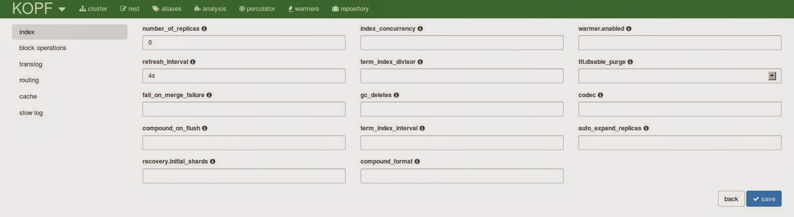
When opening the form for the index settings you will be overwhelmed at first. I didn't know there are so many settings. What is really useful is that there is an info icon next to each field that will tell you what this field is about. A great opportunity to learn about some of the settings.

What I find really useful is that you can adjust the slow index log settings directly. The slow log can also be used to log any incoming queries so it is sometimes useful for diagnostic purposes.

Finally, back on the cluster page, you can get more detailed information on the nodes or shards when clicking on them. This will open a lightbox with more details.

REST

The rest menu entry on top brings you to another view which is similar to the one Sense provided. You can enter queries and let them be executed for you. There is a request history, you have highlighting and you can format the request document but unfortunately the interface is missing the autocompletion. Nevertheless I suppose this can be useful if you don't like to fiddle with curl.

Aliases

Using the aliases tab you can have a convenient form for managing your index aliases and all the relevant additional information. You can add filter queries for your alias or influence the index or search routing. On the right side you can see the existing aliases and remove them if not needed.

Analysis

The analysis tab will bring you to a feature that is also very popular for the Solr administration view. You can test the analyzers for different values and different fields. This is a very valuable tool while building a more complex search application.

Unfortunately the information you can get from Elasticsearch is not as detailed as the one you can get from Solr: It will only contain the end result so you can't really see which tokenizer or filter caused a certain change.

Percolator

On the percolator tab you can use a form to register new percolator queries and view existing ones. There doesn't seem to be a way to do the actual percolation but maybe this page can be useful for using the percolator extensively.

Warmers

The warmers tab can be used to register index warmer queries.

Repository

The final tab is for the snapshot and restore feature. You can create repositories and snapshots and restore them. Though I can imagine that most of the people are automating the snapshot creation this can be a very useful form.

Conclusion

I hope you could see in this post that elasticsearch-kopf can be really useful. It is very unlikely that you will ever need all of the forms but it is good to have them available. The cluster view and the rest interface can be very valuable for your daily work and I guess there will be new features coming in the future.

See Your Solr Cache Sizes: Eclipse Memory Analyzer

Solr uses different caches to prevent too much IO access and calculations during requests. When indexing doesn't happen too frequently you can get huge performance gains by employing those caches. Depending on the structure of your index data and the size of the caches they can become rather large and use a substantial part of your heap memory. In this post I would like to show how you can use the Eclipse Memory Analyzer to see how much space your caches are really using in memory.

Configuring the Caches

All the Solr caches can be configured in solrconfig.xml in the query section. You will find definitions like this:

<filterCache class="solr.FastLRUCache"
  size="8000"
  initialSize="512"
  autowarmCount="0"/>

This is an example of a filter cache configured to use the FastLRUCache, a maximum size of 8000 items and no autowarming. Solr ships with two commonly used cache implementations, the FastLRUCache, that uses a ConcurrentHashMap and the LRUCache, that synchronizes the calls. Some of the caches are still configured to use the LRUCache but on some read heavy projects I had good results with changing those to FastLRUCache as well.

Additionaly, starting from Solr 3.6 there is also the LFUCache. I have never used it and it is still marked as experimental and subject to change.

Solr comes with the following caches:

FilterCache

Caches a bitset of the filter queries. This can be a very effective cache if you are reusing filters.

QueryResultCache

Stores an ordered list of the document ids for a query.

DocumentCache

Caches the stored fields of the Lucene documents. If you have large or many fields this cache can become rather large.

FieldValueCache

A cache that is mainly used for faceting.

Additionaly you will see references to the FieldCache which is not a cache managed by Solr and can not be configured.

In the default configuration Solr only caches 512 items per cache which can often be too small. You can see the usage of your cache in the administration view of Solr in the section Plugin/Stats/Caches of your core. This will tell you the hit rate as well as the evictions for your caches.

The stats are a good starting point for tuning your caches but you should be aware that by setting the size too large you can see some unwanted GC activity. That is why it might be useful to look at the real size of your caches in memory instead of the item count alone.

Eclipse MAT

Eclipse MAT is a great tool for looking at your heap in memory and see which objects occupy the space. As the name implies it is based on Eclipse and can either be downloaded as a standalone tool or is available via update sites for integration in an existing instance.

Heap dumps can be aquired using the tool directly but you can also open existing dumps. On opening it will automatically calculate a chart of the largest objects that might already contain some of the cache objects, if you are keeping lots of items in the cache.

Using the links below the pie chart you can also open further automatic reports, e.g. the Top Consumers, a more detailed page on large objects.

Even if you do see some of the cache classes here, you can't really see which of the caches it is that consumes the memory. Using the Query Browser menu on top of the report you can also list instances of classes directly, no matter how large those are.

We are choosing List Objects with outgoing references and enter the class name for the FastLRUCache, org.apache.solr.search.FastLRUCache. For the default configuration you will see two instances. When clicking on one of the instances you can see the name of the cache in the lower left window, in this case the filter cache.

There are two numbers available for the heap size: The shallow size and the retained size. When looking at the caches we are interested in the retained size as this is the size that would be available when the instance is garbage collected, i.e. the size of the cache that is only used by the cache. In our case this is around 700kB but this can grow a lot.

You can also do the same inspection for the org.apache.solr.search.LRUCache to see the real size of your caches.

Conclusion

The caches can get a lot bigger than in our example here. Eclipse Memory Analyzer has helped me a lot already to see if there are any problems with a heap that is growing too large.

What Is Special About This? Significant Terms in Elasticseach

I have been using Elasticsearch a few times now for doing analytics of twitter data for conferences. Popular hashtags and mentions that can be extraced using facets can show what is hot at a conference. But you can go even further and see what makes each hashtag special. In this post I would like to show you the significant terms aggregation that is available with Elasticsearch 1.1. I am using the tweets of last years Devoxx as those contain enough documents to play around.

Aggregations

Elasticsearch 1.0 introduced aggregations, that can be used similar to facets but are far more powerful. To see why those are useful let's take a step back and look at facets, that are often used to extract statistical values and distributions. One useful example for facets is the total count of a hashtag:

curl -XGET "http://localhost:9200/devoxx/tweet/_search" -d'
{
    "size": 0,  
    "facets": {
       "hashtags": {
          "terms": {
             "field": "hashtag.text",
             "size": 10,
             "exclude": [
                "devoxx", "dv13"
             ]
          }
       }
    }
}'

We request a facet called hashtags that uses the terms of hashtag.text and returns the 10 top values with the counts. We are excluding the hashtags devoxx and dv13 as those are very frequent. This is an excerpt of the result with the popular hashtags:

   "facets": {
      "hashtags": {
         "_type": "terms",
         "missing": 0,
         "total": 19219,
         "other": 17908,
         "terms": [
            {
               "term": "dartlang",
               "count": 229
            },
            {
               "term": "java",
               "count": 216
            },
            {
               "term": "android",
               "count": 139
            },
    [...]

Besides the statistical information we are retrieving here facets are often used for offering a refinement on search results. A common use is to display categories or features of products on eCommerce sites for example.

Starting with Elasticsearch 1.0 you can have the same behaviour by using one of the new aggregations, in this case a terms aggregation:

curl -XGET "http://localhost:9200/devoxx/tweet/_search" -d'
{
    "size" : 0,
    "aggs" : {
        "hashtags" : {
            "terms" : { 
                "field" : "hashtag.text", 
                "exclude" : "devoxx|dv13"
            }
        }
    }
}'

Instead of requesting facets we are now requesting a terms aggregation for the field hashtag.text. The exclusion is now based on a regular expression instead of a list. The result looks similar to the facet return values:

   "aggregations": {
      "hashtags": {
         "buckets": [
            {
               "key": "dartlang",
               "doc_count": 229
            },
            {
               "key": "java",
               "doc_count": 216
            },
            {
               "key": "android",
               "doc_count": 139
            },
    [...]

Each value forms a so called bucket that contains a key and a doc_count.

But aggregations not only are a replacement for facets. Multiple aggregations can be combined to give more information on the distribution of different fields. For example we can see the users that used a certain hashtag by adding a second terms aggregation for the field user.screen_name:

curl -XGET "http://localhost:9200/devoxx/tweet/_search" -d'
{
    "size" : 0,
    "aggs" : {
        "hashtags" : {
            "terms" : { 
                "field" : "hashtag.text", 
                "exclude" : "devoxx|dv13"
            },
            "aggs" : {
                "hashtagusers" : {
                    "terms" : {
                        "field" : "user.screen_name"
                    }
                }
            }
        }
    }
}'

Using this nested aggregation we now get a list of buckets for each hashtag. This list contains the users that used the hashtag. This is a short excerpt for the #scala hashtag:

 
               "key": "scala",
               "doc_count": 130,
               "hashtagusers": {
                  "buckets": [
                     {
                        "key": "jaceklaskowski",
                        "doc_count": 74
                     },
                     {
                        "key": "ManningBooks",
                        "doc_count": 3
                     },
    [...]

We can see that there is one user that is responsible for half of the hashtags. A very dedicated user.

Using aggregations we can get information that we were not able to get with facets alone. If you are interested in more details about aggregations in general or the metrics aggregations I haven't touched here, Chris Simpson has written a nice post on the feature, there is a nice visual one at the Found blog, another one here and of course there is the official documentation on the Elasticsearch website.

Significant Terms

Elasticsearch 1.1 contains a new aggregation, the significant terms aggregation. It allows you to do something very useful: For each bucket that is created you can see the terms that make this bucket special.

Significant terms are calculated by comparing a foreground frequency (which is the frequency of the bucket you are interested in) with a background frequency (which for Elasticsearch 1.1 always is the frequency of the complete index). This means it will collect any results that have a high frequency for the current bucket but not for the complete index.

For our example we can now check for the hashtags that are often used with a certain mention. This is not the same that can be done with the terms aggregation. The significant terms will only return those terms that are occuring often for a certain user but not as frequently for all users. This is what Mark Harwood calls the uncommonly common.

curl -XGET "http://localhost:9200/devoxx/tweet/_search" -d'
{
    "size" : 0,
    "aggs" : {
        "mentions" : {
            "terms" : { 
                "field" : "mention.screen_name" 
            },
            "aggs" : {
                "uncommonhashtags" : {
                    "significant_terms" : {
                        "field" : "hashtag.text"
                    }
                }
            }
        }
    }
}'

We request a normal terms aggregation for the mentioned users. Using a nested significant_terms aggregation we can see any hashtags that are often used with the mentioned user but not so often in the whole index. This is a snippet for the account of Brian Goetz:

            {
               "key": "BrianGoetz",
               "doc_count": 173,
               "uncommonhashtags": {
                  "doc_count": 173,
                  "buckets": [
                     {
                        "key": "lambda",
                        "doc_count": 13,
                        "score": 1.8852860861614915,
                        "bg_count": 33
                     },
                     {
                        "key": "jdk8",
                        "doc_count": 8,
                        "score": 0.7193691737111163,
                        "bg_count": 32
                     },
                     {
                        "key": "java",
                        "doc_count": 21,
                        "score": 0.6601749139630457,
                        "bg_count": 216
                     },
                     {
                        "key": "performance",
                        "doc_count": 4,
                        "score": 0.6574225667412876,
                        "bg_count": 9
                     },
                     {
                        "key": "keynote",
                        "doc_count": 9,
                        "score": 0.5442707998673785,
                        "bg_count": 52
                     },
        [...]

You can see that there are some tags that are targeted a lot at the keynote by Brian Goetz and are not that common for the whole index.

Some more ideas what we could look at with the significant terms aggregation:

• Find users that are using a hashtag a lot.
• Find terms that are often used with a certain hashtag.
• Find terms that are used by a certain user.
• ...

Besides these impressive analytics feature significant terms can also be used for search applications. A useful example is given in the Elasticsearch documentation itself: If a user searches for "bird flu" automatically display a link to a search to H5N1 which should be very common in the result documents but not in the whole of the corpus.

Conclusion

With significant terms Elasticsearch has again added a feature that might very well offer surprising new applications and use cases for search. Not only is it important for analytics but it can also be used to improve classic search applications. Mark Harwood has collected some really interesting use cases on the Elasticsearch blog. If you'd like to read another post on the topic you can see this post at QBox-Blog that introduces significant terms as well as the percentile and cardinality aggregations.

The Absolute Basics of Indexing Data

Ever wondered how a search engine works? In this post I would like to show you a high level view of the internal workings of a search engine and how it can be used to give fast access to your data. I won't go into any technical details, what I am describing here holds true for any Lucene based search engine, be it Lucene itself, Solr or Elasticsearch.

Input

Normally a search engine is agnostic to the real data source of indexing data. Most often you push data into it via an API that already needs to be in the expected format, mostly Strings and data types like integers. It doesn't matter if this data originally resides in a document in the filesystem, on a website or in a database.

Search engines are working with documents that consist of fields and values. Though not always used directly you can think of documents as JSON documents. For this post imagine we are building a book database. In our simplified world a book just consists of a title and one or more authors. This would be two example documents:

{
    "title" : "Search Patterns",
    "authors" : [ "Morville", "Callender" ],
}
{
    "title" : "Apache Solr Enterprise Search Server",
    "authors" : [ "Smiley", "Pugh" ]
}

Even though the structure of both documents is the same in our case, the format of the document doesn't need to be fixed. Both documents could have totally different attributes, nevertheless both could be stored in the same index. In reality you will try to keep the documents similar, after all, you need a way to handle the documents in your application.

Lucene itself doesn't even have the concept of a key. But of course you need a key to identify your documents when updating them. Both Solr and Elasticsearch have ids that can either be chosen by the application or be autogenerated.

Analyzing

For every field that is indexed a special process called analyzing is employed. What it does can differ from field to field. For example, in a simple case it might just split the terms on whitespace and remove any punctuation so Search Patterns would become two terms, Search and Patterns.

Index Structure

An inverted index, the structure search engines are using, is similar to a map that contains search terms as key and a reference to a document as value. This way the process of searching is just a lookup of the term in the index, a very fast process. Those might be the terms that are indexed for our example documents.

Field	Term	Document Id
title	Apache	2
	Enterprise	2
	Patterns	1
	Search	1,2
	Server	2
	Solr	2
author	Callender	1
	Morville	1
	Pugh	2
	Smiley	2

A real index contains more information like position information to enable phrase queries and frequencies for calculating the relevancy of a document for a certain search term.

As we can see the index holds a reference to the document. This document, that is also stored with the search index, doesn't necessarily have to be the same as our input document. You can determine for each field if you would like to keep the original content which is normally controlled via an attribute named stored. As a general rule, you should have all the fields stored that you would like to display with the search results. When indexing lots of complete books and you don't need to display it in a results page it might be better to not store it at all. You can still search it, as the terms are available in the index, but you can't access the original content.

More on Analyzing

Looking at the index structure above we can already imagine how the search process for a book might work. The user enters a term, e.g. Solr, this term is then used to lookup the documents that contain the term. This works fine for cases when the user types the term correctly. A search for solr won't match for our current example.

To mitigate those difficulties we can use the analyzing process already mentioned above. Besides the tokenization that splits the field value into tokens we can do further preprocessing like removing tokens, adding tokens or modifying tokens (TokenFilter).

For our book case it might at first be enough to do lowercasing on the incoming data. So a field value Solr will then be stored as solr in the index. To enable the user to also search for Solr with an uppercase letter we need to do analyzing for the query as well. Often it is the same process that is used for indexing but there are also cases for different analyzers.

The analyzing process not only depends on the content of the documents (field types, language of text fields) but also on your application. Take one common scenario: Adding synonyms for terms to the index. You might think that you just take a huge list of synonyms like WordNet and add those to each of your application. This might in fact decrease the search experience of your users as there are too many false positives. Also, for certain terms of the domain of your users WordNet might not contain the correct synonyms at all.

Duplication

When designing the index structure there are two competing forces: Often you either optimize for query speed or for index size. If you have a lot of data you probably need to take care that you only store data that you really need and even only put terms in the index that are necessary for lookups. Oftentimes for smaller datasets the index size doesn't matter that much and you can design your index for query performance.

Let's look at an example that can make sense for both cases. In our book information system we would like to display an alphabetic navigation for the last name of the author. If the user clicks on A, all the books of authors starting with the letter A should be displayed. When using the Lucene query syntax you can do something like this with its wildcard support: Just issue a query that contains the letter the user clicked and a trailing *, e.g. a*.

Wildcard queries have become very fast with recent Lucene versions, nevertheless it still is a query time impact. You can also choose another way. When indexing the data you can add another field that just stores the first letter of the name. This is what the relevant configuration might look like in Elasticsearch but the concept is the same for Lucene and Solr:

"author": {
    "type": "multi_field",
    "fields": {
        "author" : {
            "type": "string"
        },
        "letter" : {
            "type": "string",
            "analyzer": "single_char_analyzer"
        }
    }
}

Under the hood, another term dictionary for the field author.letter will be created. For our example it will look like this:

Field	Term	Document Id
author.letter	C	1
	M	1
	P	2
	S	2

Now, instead of issuing a wildcard query on the author field we can directly query the author.letter field with the letter. You can even build the navigation from all the terms in the index using techniques like faceting the extract all the available terms for a field from the index.

Conclusion

These are the basics of the indexing data for a search engine. The inverted index structure makes searching really fast by moving some processing to the indexing phase. When we are not bound by any index size concerns we can design our index for query performance and add additional fields that duplicate some of the data. This design for queries is what makes search engines similar to how lots of the NoSQL solutions are used.

If you'd like to go deeper in the topics I recommend watching the talk What is in a Lucene index by Adrien Grand. He shows some of the concepts I have mentioned here (and a lot more) but also how those are implemented in Lucene.